Приобретая все больше поклонников, на сегодня становятся не только проще, но и безопаснее. В нашем топе мы рассмотрим самые маленькие вертолеты в мире
.
1
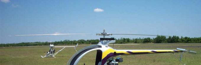
Вертолет GEN H-4 (Япония)
На сегодня это — самый маленький вертолет в мире, что засвидетельствовано даже в Книге Рекордов Гиннеса. GEN H-4, созданный одноименной японской компанией, имеет лопасти длиной 4 метра и вес всего лишь в 70 кг. У этого вертолета нет хвоста, т.к. он оснащен винтами соосного принципа действия, и это позволило значительно уменьшить его размеры. Грузоподъемность этого «малыша» впечатляет – он способен летать с весом в 210 кг (то есть ровно втрое больше собственного весе). Продаваться вертолет будет в разобранном виде, как конструктор, и, по замыслу производителей, будет собираться владельцем за 30 часов. Предложение более чем интересное, а что касается стоимости, то предположительно она будет начинаться с 200 тыс. долларов США.
2 Вертолет

На второе место мы ставим именно этот вертолет. Название уже говорит само за себя – «Москит»! Его разработка велась почти 10 лет, и «Москит» соединил в себе высокую надежность и легкость в управлении с маленькими размерами и очень хорошей маневренностью. Двигатель вертолета мощностью в 60 л.с. и 5-тиметровые лопасти с легкость поднимают в воздух машину и пилота общим весом до 300 кг. При этом сама машина весит всего 115 кг. Стоимость этой машины и ее модификаций стартует от 40 тыс. долларов.
3 Вертолет

Впервые этот вертолет взлетел в 2004 году, и изначально задумывался для экстремальных забав. Но на сегодня он и патрульный, пограничный, почтовый, а также учебный, поскольку, как оказалось, он имеет хорошие летные характеристики и очень надежен в использовании. Вес AirScooter II — всего 136 кг, объем двигателя — 65 л.с., скорость — 90 км/ч, потолок – 3 тыс. метров. На сегодня этот аппарат «разлетелся» (во всех смыслах) в 23 страны по цене в 50 тыс. долларов за единицу.
4 Вертолет

Этот легкий двухместный вертолет впервые поднялся в воздух в 2004 году. Он также мал и максимально удобен в эксплуатации, имеет высокие летные характеристики. Двигатель в 130 л.с. разгоняет машину до 160 км/ч на высоту в 3,6 км. Диаметр винта — 7 метров, грузоподъемность — 230 кг. Поставляется в разобранном виде, сборка требует около 250 часов. Стоимость вертолета составляет 95 тыс. евро.

Итальянцы также стараются не отставать в малой авиации. Они изготовили и продали уже более 400 своих сверхлегких вертолетов марки СН-7. Популярность он стал приобретать практически сразу с момента своего производства в 1996 году. Диаметр винта — 5,8 м., вес — 200 кг, максимальная скорость – 192 км/ч. В некоторых модификациях стоимость аппарата достигает 85-90 тыс. евро.
6 Вертолет

Легкий вертолет этой марки можно смело назвать «дедушкой» современных сверхлегких вертолетов. Созданный еще в 1975 году, он существует в более чем 3 тыс. экземпляров, эксплуатируемых в 60-ти странах мира. Основная масса современных вертолетов использует в своих конструкциях решения, найденные именно в R22. Сегодня этот вертолет стоит 258 тыс. долларов.
7 Вертолет DF Helicopters DF334 (Италия)

Двухместный сверхлегкий вертолет, также разработанный уже довольно давно — в 1980-х годах, за это время только подтвердивший свою надежность (вот уж точно, «в бой идут одни старики»…). Вес — всего 290 кг., винт – 6,8 м., скорость — 148 км/ч, стоимость — от 120 тыс. евро.
8 Вертолет Skyline SL-222 (Украина)

Легкий многоцелевой вертолет, который производится с 2011 года. Так же, как и его «собратья», может транспортироваться на обычном автоприцепе, прост и надежен в эксплуатации. Вес составляет 377 кг, стоимость — 149 тыс. долларов.
9 Вертолет

С 2003 года именно эта машина стала одной из самых популярных в своем классе. С весом всего в 445 кг и скоростью в 185 км/ч «EXEC» поднимается на 3048 м. Стоимость — от 280 тыс. долларов.
10 Вертолет Беркут-ВЛ (Россия)

Сегодня разработка этого вертолета находится в стадии окончательных испытаний, но имеет хорошие перспективы развития. Двигатель в 140 л.с. поднимает 477 кг (вес вертолета) на высоту в 4 км и развивает скорость в 185 км/ч. В скором времени ждем достойного представителя России на рынке легкой авиации!
Легкая авиация может воплотить мечту каждого человека о полете. И мы видим, что на сегодня уже существуют вертолеты стоимостью с хороший автомобиль. Поэтому очень вероятно, что в скором времени появятся и более доступные аппараты, а может быть, и еще меньших размеров!
Решили изучить OpenGL, но знаете, с чего начать? Сделали подборку материалов.
Что есть OpenGL
OpenGL (открытая графическая библиотека) - один из наиболее популярных графических стандартов для работы с графикой. Программы, написанные с её помощью можно переносить практически на любые платформы, получая одинаковый результат. OpenGL позволяет не писать программы под оборудование, а воспользоваться существующими разработками. Разрабатывает OpenGL компания Silicon Graphics, при сотрудничестве с другим технологическими гигантами.
С точки зрения программирования, OpenGL - это программный интерфейс для растровой графики, таких как графические ускорители. Он включает в себя около 150 различных команд, с помощью которых программист может определять различные объекты и производить рендеринг.
Материалы для изучения
Туториалы
Онлайн-курсы
- Lynda - «Курс по OpenGL»;
- Токийский университет - «Интерактивная компьютерная графика»;
- Университет Сан-Диего - «Основы компьютерной графики».
Книги
На русском
1. Д. Шрайнер - OpenGL Redbook - скачать;
Книга - официальное руководство по изучению OpenGL. Последние издания практически полностью отличаются от первоначальных вариантов, автор обновляет её в соответствии с изменениями версий. По мнению сотен специалистов, работающих с Open GL, эта книга является первым, что должен взять в руки желающий изучить технологию.
2. Д. Вольф - Open GL 4. Язык шейдеров. Книга рецептов (2015) - скачать;

В этой книге рассматривается весь спектр приемов программирования на GLSL, начиная с базовых видов шейдеров – вершинных и фрагментных, – и заканчивая геометрическими, вычислительными и шейдерами тесселяции. Прочтя ее, вы сможете задействовать GPU для решения самых разных задач.
3. Д. Гинсбург - OpenGL ES 3.0. Руководство разработчика (2014) - купить;

В данной книге автор рассматривает весь API и язык для написания шейдеров. Также вы найдете советы по оптимизации быстродействия, максимизации эффективности работы API и GPU и полном использовании OpenGL ES в широком спектре приложений.
4. В. Порев - Компьютерная графика (2002) - скачать;

В книге рассмотрены способы работы с компьютерной графикой, частые проблемы, приведены примеры программ на C++.
На английском
1. П. Ширли - Основы компьютерной графики (2009) - ;

Книга предназначена для введение в компьютерную графику на базовом уровне. Авторы рассказывают про математические основы компьютерной графики с акцентом на то, как применять эти основы для разработки эффективного кода.
2. Э. Ангел - Интерактивная компьютерная графика - купить ;

Эта книга предназначена для всех студентов, изучающих информатику и программирование углубленно. Компьютерная анимация и графика - уже не так сложно, как раньше. Следуя своему утверждению, автор написал книгу максимально понятным языком.
When I first began looking into OpenGL with Python, my main goal was to figure out how to make a rotating cube. I don"t think I am alone, since this seems to be the pinnacle of understanding the basics of OpenGL. As such, I have compiled this first video to include everything from acquiring Python , and PyGame , to creating the necessary code to make a rotating cube. This first tutorial is quite long, but I wanted to go ahead and put everything into this video. I had a very hard time figuring out OpenGL, mainly because most of the OpenGL with PyOpenGL tutorials that I could find were clearly written for someone who already knew OpenGL. I did not, so this was a massive hurdle for me. Hopefully I can help you all learn it much faster than I did.
First off, PyOpenGL is just some Python bindings (some Python code that acts like a sort of wrapper around native code), so you can manipulate OpenGL within the context of Python. OpenGL is a cross-language API, so you can take your knowledge of OpenGL to other languages.
So, the way OpenGL works is you just specify the objects within space. For a cube, for example, you specify the "corners." Corners are referred to as vertices (plural) or as a vertex (singular). You may also see them referred to as a node (singular) or nodes (plural).
Once you define the vertices, you can then do things with them. In this example, we want to draw lines between them. Defining the vertices is done with a simple list or tuple in Python. You can then pre-define some rules like what vertices make up a "surface" and between what vertices are the "edges," or lines that we want to have drawn between the vertices.
Once you do that, then you"re ready to write the OpenGL code. To do this, you have glBegin and glEnd statements that you call, and between these is where the OpenGL-specific code goes. In the glBegin statement, you specify the "type" of code that you are about to pass. These are constants, and contain things like GL_QUADS or GL_LINES. This basically notifies OpenGL how you want it to handle your statements.
So that"s the abstract concept of how OpenGL works, let"s go ahead and do it!
Next, we import OpenGL.GL and OpenGL.GLU. OpenGL.GL is just your typical OpenGL functions, then OpenGL.GLU is some of the more "fancy" OpenGL functions.
For the first few videos, I go ahead and miss-spell vertices. Oops.
Vertices= ((1, -1, -1), (1, 1, -1), (-1, 1, -1), (-1, -1, -1), (1, -1, 1), (1, 1, 1), (-1, -1, 1), (-1, 1, 1))
Here, we"ve defined the location (x,y,z) of each vertex. I think it is best to envision this in "units." Try to think of these locations "spatially." With a cube, there are 8 "nodes" or vertices.
Next, we"re ready to define the edges:
Edges = ((0,1), (0,3), (0,4), (2,1), (2,3), (2,7), (6,3), (6,4), (6,7), (5,1), (5,4), (5,7))
Each of the above tuples contains two numbers. Those numbers correspond to a vertex, and the "edge" is going to be drawn between those two vertices. We start with 0, since that"s how Python and most programming languages work (the first element is 0). So, 0 corresponds to the first vertex we defined (1, -1, -1)... and so on.
Now that we"ve got that, let"s work on the required code to work with OpenGL to actually generate a cube:
Def Cube(): glBegin(GL_LINES) for edge in edges: for vertex in edge: glVertex3fv(vertices) glEnd()
First, we start off our function as we would any other function.
Next, since this is just a function containing OpenGL code, we go ahead and open with a glBegin(GL_LINES), this notifies OpenGL that we"re about to throw some code at it, and then the GL_LINES tells OpenGL how to handle that code, which, in this case, means it will treat the code as line-drawing code.
From there, we say for edge in edges, which corresponds to each pair of vertices in our edges list. Since each edge contains 2 vertices, we then say for vertex in edge, do glVertex3fv(vertices), which performs the glVertex3fv OpenGL function on the element of the vertices tuple.
As such, what ends up being passed through OpenGL with the constant of GL_LINES is:
glVertex3fv((1, -1, -1))
glVertex3fv((1, 1, -1))
And so on. OpenGL, knowing that we"re drawing lines here will draw lines between those points.
After running through all edges, we"re done, so we call glEnd() to notify OpenGL that we"re done telling it what to do. For each "type" of OpenGL code that you plan to use, you will need opening and closing GL commands like this.
That"s it for our cube function. This function will create the cube, but now we want to display the cube and specify our perspective in the environment:
Def main(): pygame.init() display = (800,600) pygame.display.set_mode(display, DOUBLEBUF|OPENGL)
This is mostly typical PyGame code. If you want to understand it more, check out the .
The only major difference here is we"re adding another "parameter" looking thing after "display" in the pygame.display.set_mode. These are actually constants, notifying PyGame that we"re going to be feeding it OpenGL code, as well as DOUBLEBUF, which stands for double buffer, and is a type of buffering where there are two buffers to comply with monitor refresh rates. Take note that pipe ("|") that is used to separate constants. It will be used again later to separate constants.
Next, within this main() function:
GluPerspective(45, (display/display), 0.1, 50.0)
gluPerspective is code that determines the perspective, as it sounds. The first value is the degree value of the field of view (fov). The second value is the aspect ratio, which is the display width divided by the display height. The next two values here are the znear and zfar, which are the near and far clipping planes.
What in the heck is a clipping plane? If you"re like me, that means nothing to you at this point. Basically, a clipping plane is at what distance does the object appear/disappear. So the object will only be visible between these two values, and both values are supposed to be positive, because they are in relation to your perspective, not in relation to your actual location within the 3D environment.
So, we"re having the close clipping happening at 0.1 units and the far clipping plane as 50.0 units away. This will make more sense later, once we"ve displayed the cube and we can control where we are in the 3D environment, then you will see the clipping planes in action.
Next up, we have:
GlTranslatef(0.0,0.0, -5)
glTranslatef, officially "multiplies the current matrix by a translation matrix." OK cool, again that means nothing to me. So, in layman"s terms, this basically moves you, and the parameters are x, y and z. So above, we"re moving back 5 unites. This is so we can actually see the cube when we bring it up. Otherwise, we"d be a bit too close.
Now let"s write our typical event loop for PyGame. Again, if you want to learn more, check out the aforementioned tutorial.
While True: for event in pygame.event.get(): if event.type == pygame.QUIT: pygame.quit() quit()
This is a simple PyGame event loop that is only checking for any exit, which is only looking for the literal "x" out. Continuing under this "while" statement:
GlRotatef(1, 3, 1, 1) glClear(GL_COLOR_BUFFER_BIT|GL_DEPTH_BUFFER_BIT) Cube() pygame.display.flip() pygame.time.wait(10)
glRotatef multiplies the current matrix by a rotation matrix. The parameters here are angle, x, y and z.
Then we have glClear, which is like any other clearing function. We specify a couple of constants here, which is telling OpenGL what exactly we"re clearing.
Once we have a clean "canvas" if you will, we then call our Cube() function.
After that, we call pygame.display.flip(), which updates our display.
Finally we throw in a short wait with pygame.time.wait(10).
That"s it for our main function, and now we just call a main() at the end to make it all work. Just in case you got lost somewhere, here"s the entire script put together:
Import pygame from pygame.locals import * from OpenGL.GL import * from OpenGL.GLU import * verticies = ((1, -1, -1), (1, 1, -1), (-1, 1, -1), (-1, -1, -1), (1, -1, 1), (1, 1, 1), (-1, -1, 1), (-1, 1, 1)) edges = ((0,1), (0,3), (0,4), (2,1), (2,3), (2,7), (6,3), (6,4), (6,7), (5,1), (5,4), (5,7)) def Cube(): glBegin(GL_LINES) for edge in edges: for vertex in edge: glVertex3fv(verticies) glEnd() def main(): pygame.init() display = (800,600) pygame.display.set_mode(display, DOUBLEBUF|OPENGL) gluPerspective(45, (display/display), 0.1, 50.0) glTranslatef(0.0,0.0, -5) while True: for event in pygame.event.get(): if event.type == pygame.QUIT: pygame.quit() quit() glRotatef(1, 3, 1, 1) glClear(GL_COLOR_BUFFER_BIT|GL_DEPTH_BUFFER_BIT) Cube() pygame.display.flip() pygame.time.wait(10) main()
The end result should be:
Awesome and congratulations on your PyOpenGL cube! There is obviously a lot more to learn, and some of these functions may not make too much sense just yet. I"ll be going over those a bit more in depth soon.
This tutorial uses both.
OpenGL
Make sure you have a driver with good OpenGL support installed. On a current system OpenGL support should be well above 2.1. Check with glxinfo from mesa-progs.
glxinfo | grep -e "direct rendering:" -e "OpenGL renderer string:" \ -e "OpenGL version string:"
On my system this shows:
direct rendering: Yes OpenGL renderer string: AMD Radeon HD 6670 OpenGL version string: 4.2.12337 Compatibility Profile Context 12.104
So we are good to go here. Note: I am using the ATI drivers. The Open Source radeon driver was at OpenGL version 2.1 at the time of writing.
SDL 2.0
We need something to give us a window with a OpenGL context. Since I plan to use OpenGL in games SDL comes to mind. However the 2.0 Version is in release candidate phase . So we will compile it from source. "openglexample" is a project folder in which we will do our tests.
[ openglexample] $ curl -sS "http://www.libsdl.org/release/SDL2-2.0.0.tar.gz" | tar xvz [ openglexample] $ cd SDL2-2.0.0 [ SDL2-2.0.0] $ ./autogen.sh [ SDL2-2.0.0] $ ./configure [ SDL2-2.0.0] $ make
Now install SDL2. The library will then go into /usr/local/lib .
[ SDL2-2.0.0] $ sudo make install [ SDL2-2.0.0] $ cd ..
Remove the source if you do not need it anymore.
[ openglexample] $ rm -rf SDL2-2.0.0
Of course you may download manually or check out news about SDL first here www.libsdl.org .
PySDL2
Let"s do a quick test to see if SDL 2.0 and PySDL2 work.
(pysdl2)[ openglexample] $ python ~/.virtualenvs/pysdl2/lib64/python3.2/site-packages/sdl2/examples/sdl2hello.py
This should show a black window with "Hello World" in the title. You may have to adapt that path. Just note that there are some examples in site-packages/sdl2/examples . They will not all work right away. To make them work you will have to compile/install SDL_image , SDL_mixer , SDL_ttf , SDL_gfx and add PyOpenGL (see below)
PyOpenGL
This is the center piece of our attention. You can find out more about it on the . Please note that Python 3 support is still considered experimental. So be prepared and help improving it. There is also a package named for teaching and testing purposes as part of the PyOpenGL project. However I found that it abstracts away some parts and seems to be Python 2 only. Since all of this is a means of learning current OpenGL with GLSL and such for me it"s best to have as little abstraction as possible from the pure OpenGL structures and interfaces.
Let"s go ahead and install PyOpenGL in our virtualenv.
(pysdl2)[ openglexample] $ pip install pyopengl
At the time of writing this installed version 3.1.0a1 of PyOpenGL. Now the little opengl example, that came with PySDL2 should work. Check it out.
(pysdl2)[ openglexample] $ python ~/.virtualenvs/pysdl2/lib64/python3.2/site-packages/sdl2/examples/opengl.py
You should see a spinning triangle. Now our environment is set up and we can finally get started with our custom OpenGL code.
OpenGL with GLSL and Arrays
The example code we will produce now has one simple goal: Show a white triangle on an orange background. Orange is the background color of choice because black always has the notion that nothing worked. But we will do so using the new way of doing things in OpenGL. Namely shaders and arrays .
And at this point I owe special thanks to two distinctive sources without which I would have probably thrown in the towel.
- open.gl Looks current and an excellent starting point. It"s in targeted at C++, but I found it extremely helpful.
- Python examples from Sean J. McKiernan Even though the examples are targeted at Python 2.7 and use Pygame they were the help I needed to weed out a nasty bug that gave me no errors but no triangle either. I will point this out again further below.
Now a quick and dirty overview how this new style of OpenGL programming is organized would certainly be helpful. And here I will try not to disappoint. It very much all boils down to:
You create arrays of data such as vertices, colors, and pretty much anything you like. These are called: Vertex Buffer Objects (VBOs) .
You set up small programs in a C like language, the GLSL , which work on these VBOs one element (vertex, color, whatever) at a time. But quite likely in a massively parallel fashion. These are called Shaders .
You set up a mapping between these array elements of the VBOs and the respective, possibly self-defined, attribute names in the shaders. This is stored in Vertex Array Objects (VAOs)
Most of the setup will be done before anything is rendered. The main point is that you move as much of the data as possible over to the graphics card before any rendering or animation is done. Then at runtime, when for example a game is actually being played, you will mostly just bind and unbind VBOs and VOAs, switch the shaders which are to be used and influence some global parameters of the shaders, so called uniforms , from your program. This way you only make very light calls to the graphics card. You will only quite rarely work on arrays of stuff (vertices, colors and so forth) at runtime and almost never on actual pixel data. With this in mind I am fairly certain that Python should be fine for most applications.
The Code
We will now build our small example step-by-step. You can also find the complete file near the bottom of this post. But I recommend playing it through from the start.
Open up your favorite editor:
(pysdl2)[ openglexample] gvim example1.py
We will not do a * wildcard import here although it may seem convenient at first. But this way there will be no doubt about from where a name originates.
"""Example 1: white triangle on orange background setting up a window with OpenGL context and rendering one white triangle on an orange background using shaders """ import ctypes import sdl2 from OpenGL import GL
For this first example we will fit everything in one function.
def run (): if sdl2 . SDL_Init (sdl2 . SDL_INIT_VIDEO ) != 0 : print (sdl2 . SDL_GetError ()) return
We are now diving head on into OpenGL. Don"t worry if you don"t understand everything at once. It will become clearer when you see the whole picture.
# get Vertex Array Object name vao = GL . glGenVertexArrays (1 ) # set this new VAO to the active one GL . glBindVertexArray (vao )
Now we need to get a new VBO object from the graphics card and fill it with our data.
# get a VBO name from the graphics card vbo = GL . glGenBuffers (1 ) # bind our vbo name to the GL_ARRAY_BUFFER target GL . glBindBuffer (GL . GL_ARRAY_BUFFER , vbo ) # move the vertex data to a new data store associated with our vbo GL . glBufferData (GL . GL_ARRAY_BUFFER , ctypes . sizeof (triangle_array ), triangle_array , GL . GL_STATIC_DRAW )
You can see that it is somewhat similar to the VAO creation. There are however different types of buffers. So you have to specify which buffer should be represented by our vbo. The most interesting call is . The last parameter GL_STATIC_DRAW is just a hint on how the data will be used.
After we have specified the vertex data we need to move on to the shaders to specify how our triangle will be rendered. The 2 different types of shaders you need to think about now are:
- Vertex Shaders : compute the position and additional data for each vertex. You would do 3D transformation here.
- Fragment Shaders : computes the color of each pixel. You would for example apply your texture data here.
The vertex shader in our code is assembled like this:
# vertex shader vertexShaderProgram = """#version 100 in vec2 position; void main() { gl_Position = vec4(position, 0.0, 1.0); }""" vertexShader = GL . glCreateShader (GL . GL_VERTEX_SHADER ) GL . glShaderSource (vertexShader , vertexShaderProgram ) GL . glCompileShader (vertexShader )
The shader program is just represented as a string, then we get a new name for it (i.e. create it), attach the source string and compile it. The shader source is written in GLSL the OpenGL Shading Language. You can see the full reference here: OpenGL Shading Language . Also check out the quick reference guide and have a look at the pages with the OpenGL Pipeline . This shows you that each shader has its position in the graphics pipeline. It has some inputs, modifies the data and outputs it to the next shader.
You can see the vertex shader in our example has a 2-component vector input. Our triangle vertices will go through here. We only use 2D for now so only the x and y coordinate are used. z is set to 0.0. You can also use position.x, position.y to access the components. The coordinates x,y and z are automatically divided by the 4th component. Don"t worry about this now. Just set it to 1.0.
Note: gl_Position is a builtin output variable for vertex shaders
The version preprocessor directive indicates which version of the GLSL the shader will use. Version 1.00 which came with OpenGL 2.0 is good enough for this small example.
Furthermore it is important to know that the compilation step will not raise an exception in case compilation fails. For example due to a syntax error. The later call to will however fail. For debugging shaders have a look at the functions and .
Now we move on to the fragment shader, which will deal with the color of each pixel of our triangle.
# fragment shader fragmentShaderProgram = """#version 100 out vec4 outColor; void main() { outColor = vec4(1.0, 1.0, 1.0, 1.0); }""" fragmentShader = GL . glCreateShader (GL . GL_FRAGMENT_SHADER ) GL . glShaderSource (fragmentShader , fragmentShaderProgram ) GL . glCompileShader (fragmentShader )
The code is pretty similar to what we had for our vertex shader. Instead of a position the fragment shader does however output a color. Here the color is fixed to white (1.0 for all RGBA components). But it could just as well be sampled from a texture which I will show in later examples.
Note: You won"t find outColor in any documentation. However the first user defined output variable will be output to the default framebuffer"s default color buffer (GL_BACK here). See Default Framebuffer Wiki for more information. Or you expicitly name the fragment output with glBindFragDataLocation as we will do for completeness further below.
At this point we have the source for our 2 shaders ready and compiled. We will now attach them to a shader program. You can have a lot of different programs and switch between them at runtime.
# shader program shaderProgram = GL . glCreateProgram () GL . glAttachShader (shaderProgram , vertexShader ) GL . glAttachShader (shaderProgram , fragmentShader )
This code gives us a new empty program and then the vertex and fragment shaders are attached to it.
Next we specify where the fragment output color will come from.
# color output buffer assignment GL . glBindFragDataLocation (shaderProgram , 0 , b "outColor" )
As stated before this is not strictly necessary since the first user defined output will be taken as default. However we explicitly specify it here for completeness. 0 is the index into the array of color buffers. Check glDrawBuffers for more information. Basically you can render to more than one buffer, possible off-screen, to a texture and reuse the output elsewhere in your scene.
After this we move on to linking, validating and activating our program.
# link the program GL . glLinkProgram (shaderProgram ) # validate the program GL . glValidateProgram (shaderProgram ) # activate the program GL . glUseProgram (shaderProgram )
This very much like you would expect it from a programming language such as C. First you compile all the parts (here the shaders) then you build a program from all or a subset of the parts. Imagine how you would use this in a complicated setup with a lot of prepared shaders and then stick together a handful of programs between which you switch back and forth. For example one program for all objects in your scene with matte surface and another for all objects with a glossy surface. The validation step checks whether the program can possible run in the current OpenGL state at all.
We are getting much closer to actually getting something on the screen now. The next step is to define what parts of our vertex data, the triangle corners, will flow where into the shaders.
# specify the layout of our vertex data posAttrib = GL . glGetAttribLocation (shaderProgram , b "position" ) GL . glEnableVertexAttribArray (posAttrib ) GL . glVertexAttribPointer (posAttrib , 2 , GL . GL_FLOAT , False , 0 , ctypes . c_voidp (0 ))
The Final Result
This is what you should see when you run the program.
Not that impressive you say? But believe me it is a solid start:).
Debugging
While I will not go into explicitly OpenGL related debugging here I recommend running the example in the Python debugger. Have a look at what you get back from the OpenGL calls.
(pysdl2)[ openglexample] $ python -m pdb example1.py
A quick reminder. Press n to execute the currently displayed line and step to the next line or press s to execute the current line and step into a function call. Press just to repeat the last command. So in this case n and a bunch of times just until you see:
-> run () (Pdb )
Step into with s and then move with n. Check out the some of the fancy sounding things like the vbo .
-> GL . glBindBuffer (GL . GL_ARRAY_BUFFER , vbo ) (Pdb ) pp vbo 1 (Pdb )
You can see that things like the vbo are just identifiers or names for the objects themselves. Just simple integer numbers.
Discussion / Next Topics ?
We have barely touched the surface here. To be honest we just made sure everything works. There is a lot to explore and many directions to go in. I suggest you mess around with the code a bit to get familiar with the constructs.
Assuming that Murphy"s law holds true once more you will probably be disappointed that something did not work and you do not know where it fails.
With that in mind I plan my next post to be on debugging the OpenGL state in this very example step-by-step.